Welcome to chowclassifier’s documentation!
Module Description
Introduction
There are many application where it is useful to analyse rapidly a large number of time-series for overall trends and possible breakpoint at which the trend changes. For example, spotting increasing trends in potential contaminants concentration from the outputs of non-target screening from high resolution mass spectrometry.
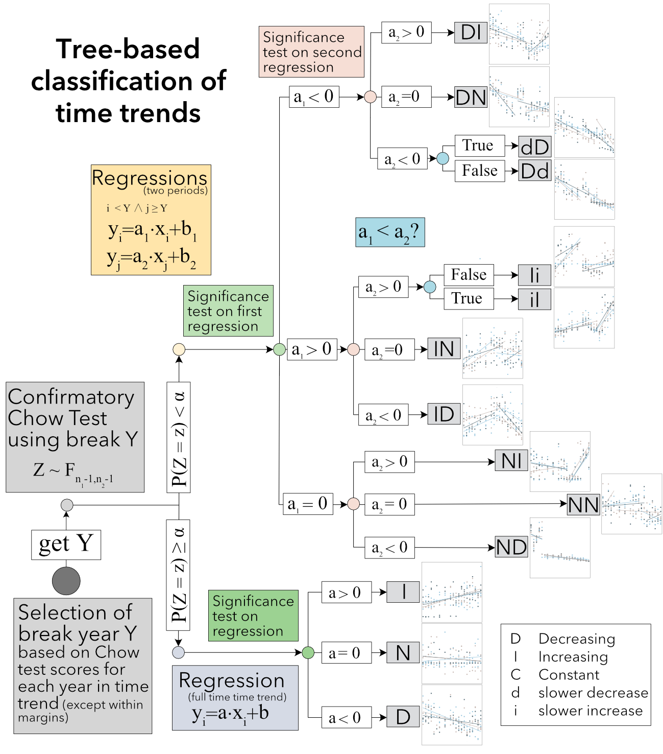
ChowClassifier aims to solve this. It is a script that performs a series of Chow tests on a time-indexed dataset to determine if a breakpoint in the time trends is probable. Two classes Chow and ChewData enable to perform the tests, generate plots and export the results in csv and excel. Dataset with groups can be ran simultaneously with ChewData indicating with namecol the name of the grouping column. Calling run on a ChewData instance will create an instance of Chow for each group and classify them into the following categories.
Breakpoint ? |
Category |
Description |
No |
N |
non-significant overall trend |
No |
I |
significant increasing overall trend |
No |
D |
significant decreasing overall trend |
Yes |
NN |
non-significant trend on set1 and non-significant trend on set2 |
Yes |
NI |
non-significant trend on set1 and significant increasing trend on set2 |
Yes |
ND |
non-significant trend on set1 ans significant decreasing trend on set2 |
Yes |
IN |
significant increasing trend on set1 and non-significant trend on set2 |
Yes |
ID |
significant increasing trend on set1 and significant decreasing trend on set2 |
Yes |
iI |
significant increasing trend on both set1 and set2 with greater increase in set2 |
Yes |
Ii |
significant increasing trend on both set1 and set2 with greater increase in set1 |
Yes |
DN |
significant decreasing trend on set1 and non-significant trend on set2 |
Yes |
DI |
significant decreasing trend on set1 and significant increasing trend on set2 |
Yes |
dD |
significant decreasing trend on both set1 and set2 with greater decrease in set2 |
Yes |
Dd |
significant decreasing trend on both set1 and set2 with greater decrease in set1 |
where set1 and set2 indicate respectively the data before the breakpoint and after. The decision process for this classification is shown in the following schema:
Chow test
Chow test was first derived by Gregory Chow [1] in 1960 and later by Franklin Fisher [2]. We test the significance of the breakpoint at level \(\alpha^\star = \frac{\alpha}{m}\) (where \(m\) is the number of breakpoints tests, thus \(\alpha^\star\) is the Bonferroni corrected significance level) under the null hypothesis \(Z=\frac{S_c-(S_1+S_2)}{S_1+S_2}\cdot\frac{N_1+N_2-2\cdot k}{k}\) where \(k=3\) is the total number of parameters. This follows a F-distribution with \(k\) and \(N_1+N_2-6\) degrees of freedom, where \(S_C`\) is the sum of squared residuals of the regression on the full time series, \(S_1\), \(S_2\) are the sums of squared residuals of the regression on the first, and respectively, the second half of the time series and \(N_1\), \(N_2\) are the number of observation for each half. See also [3].
References
Installation
Use the following command to install chowlcassifier:
pip install chowclassifier
Citation
If you use this package in your research, please cite:
Influence of Season on Biodegradation Rates in Rivers
Run Tian, Malte Posselt, Luc T. Miaz, Kathrin Fenner, and Michael S. McLachlan
Environmental Science & Technology 2024 58 (16), 7144-7153
Use
The script can be ran on any file with python -m chowclassifier -f path/to/file/filename.csv -X xcol -y ycol -n grouping_name or it can be imported:
from chowclassifier import ChewData
# define the path to data
filepath = "example/data"
# define the name of the file containing the data (with extension)
filename = "stocks.csv"
# define the path where figures will be saved
savingpath_figures = 'example/fig'
# what name has the X/time column?
timecol = 'Date'
# what name has the y/value column?
ycol = 'Close'
# what level of confidence? Note, when
# testing multiple breakpoint, a Bonferroni correction will be applied
alpha = 0.01
# initial breakpoint ?
initial_breakpoint = None

C = ChewData(filename = f"{'/'.join([x for x in [filepath,filename] if x not in [None,'']])}",
            timecol = timecol,# name of time column (used as x-axis)
            ycol = ycol,# name for value column (used as y-axis) Leave blank if multiple
            alpha = alpha# level of confidence to use
            )

########## use the code line below if your X/time column is not a number, e.g. a date
########## comment it otherwise
# C.parse_timecol(date_format = '%Y-%m-%d') #

C.run(initial_breakpoint = initial_breakpoint)
C.plot(xlabel = 'time',# label for x axis
      ylabel='value',# label for y axis
      title = "Chow Classification",# title of the main plot
      filename = f"{'/'.join([x for x in [savingpath_figures,filename] if x not in [None,'']])}.png",# filename for the figure
      figsize=(16,8),# figure size
      sharey=True # whether the individual plots are forced to share y axis
      )
C.plot_individually(savingpath = savingpath_figures,# Saving path for the figures
                  format = 'png',# figure format
                  xlabel = 'time',# label for x axis
                  ylabel='value',# label for y axis
                  )

C.plot_by_group('g',
               savingpath = savingpath_figures,# Saving path for the figures
               format = 'png',# figure format
               xlabel = 'time',# label for x axis
               ylabel='value',# label for y axis
               plot_overall = True,# Whether to plot an overall trend across groups (including confidence inverval fill)
               plot_individual_fill = True# Whether to plot individual confidence inverval fills
               )
Class and method descriptions
Licence
GNU LESSER GENERAL PUBLIC LICENSE Version 2.1, February 1999
Outputs
plot and plot_individually
Both methods, plot the best models (either the regression on the whole dataset or, two separate regressions on the left and right parts of the dataset split at breakpoint) for all subdatasets (either each in individual files or together). The filled area represents the confidence interval for the predicted values in the regression model/models. The scatter points show the observed data. The lines are the regression lines.
save_to_file
The output’s columns are described in the following table. model0 correspond to the regression on the whole dataset. model1 and model2 correspond to regressions on respectively the left and right parts of the dataset split at the breakpoint.
Model |
property |
Description of the property |
|---|---|---|
Global |
name |
Name of the group |
Global |
breakpoint |
Significant breakpoint (if found) |
Global |
score |
lowest p-value over the tested breakpoints |
model0 |
intercept |
intercept |
model0 |
slope |
slope |
model0 |
R2 |
coefficient of determination |
model0 |
se_intercept |
standard error for the intercept |
model0 |
se_slope |
standard error for the slope |
model0 |
n |
number of data points used in the fit |
model0 |
intercept_pvalue |
p-value of the intercept |
model0 |
slope_pvalue |
p-value of the slope |
model0 |
intercept_ci_lower |
lower bound of the confidence interval of the intercept |
model0 |
intercept_ci_upper |
upper bound of the confidence interval of the intercept |
model0 |
slope_ci_lower |
lower bound of the confidence slope of the intercept |
model0 |
slope_ci_upper |
upper bound of the confidence interval of the slope |
alpha |
significance level at which the regressions were tested |
|
alpha_Bonferroni_corrected |
Bonferroni corrected significance level at which the breakpoints were tested |
|
model1 |
intercept |
intercept |
model1 |
slope |
slope |
model1 |
R2 |
coefficient of determination |
model1 |
se_intercept |
standard error for the intercept |
model1 |
se_slope |
standard error for the slope |
model1 |
n |
number of data points used in the fit |
model1 |
intercept_pvalue |
p-value of the intercept |
model1 |
slope_pvalue |
p-value of the slope |
model1 |
intercept_ci_lower |
lower bound of the confidence interval of the intercept |
model1 |
intercept_ci_upper |
upper bound of the confidence interval of the intercept |
model1 |
slope_ci_lower |
lower bound of the confidence slope of the intercept |
model1 |
slope_ci_upper |
upper bound of the confidence interval of the slope |
alpha |
significance level at which the regressions were tested |
|
alpha_Bonferroni_corrected |
Bonferroni corrected significance level at which the breakpoints were tested |
|
model2 |
intercept |
intercept |
model2 |
slope |
slope |
model2 |
R2 |
coefficient of determination |
model2 |
se_intercept |
standard error for the intercept |
model2 |
se_slope |
standard error for the slope |
model2 |
n |
number of data points used in the fit |
model2 |
intercept_pvalue |
p-value of the intercept |
model2 |
slope_pvalue |
p-value of the slope |
model2 |
intercept_ci_lower |
lower bound of the confidence interval of the intercept |
model2 |
intercept_ci_upper |
upper bound of the confidence interval of the intercept |
model2 |
slope_ci_lower |
lower bound of the confidence slope of the intercept |
model2 |
slope_ci_upper |
upper bound of the confidence interval of the slope |
alpha |
significance level at which the regressions were tested |
|
alpha_Bonferroni_corrected |
Bonferroni corrected significance level at which the breakpoints were tested |
Version changes
1.1.1 |
Fixed empty unused plots, added breakpoint-margin constraints, added test example, added CI. |
1.0.10 |
Minor addition, with show_legend option |
1.0.9 |
Correction of bugs, added jupyter notebook example. |
1.0.8 |
Correction of bugs. |
1.0.7 |
Split main classes and utilities in multiple files, added option to ChewData.plot to have grouped trends, corrected input parsing, corrected inconsistancy with intial_breakpoint/margin. Added option to change linestyle by trend individually |
1.0.5 |
Added option to plot confidence interval fill for individual group trends |
1.0.4 |
Added support for plotting individual trends by group |
1.0.3 |
Bug correction |
1.0.2 |
Added support to parse full csv/excel automatically |
1.0.1 |
First implementation of algorithm |